Table of Contents
Introduction
This software package is developed for the analysis of data collected in DRAGON experiments at TRIUMF. The software is intended for experiments run with the "new" (c. 2013) DRAGON data acquisition system (VME hardware + timestamp coincidence matching).
At its core, the package is simply a collection of routines to extract ("unpack") the MIDAS data generated during an experiment into a format that is more suitable for human consumption, as well as to perform some of the more basic and commonly needed analysis tasks. From here, users can further process the data using their own codes, or they can interface with a visualization library to view the data in histograms, either online or offline. The core of the package is written in "plain" C++, that is without any dependence on libraries other than the standard library.
In addition to the "core", this package also includes code to interface with the rootana data analysis package distributed as part of MIDAS and the rootbeer program for data visualization. Each of these packages is designed for "user friendly" viewing of data in histograms, either from saved files or real-time online data. Both require that a relatively recent version of ROOT be installed on your system, and, additionally, MIDAS must be installed in order to look at online data (offline data viewing should be possible without a MIDAS installation, however). In addition, it is required that ROOT be build with the minuit2 and xml options set to ON.
There is also an optional extension to create python wrappers for the DRAGON classes, allowing data to be analyzed in python independent of ROOT/PyRoot. This package is somewhat in the experimental stage at the moment and requires installation of Boost.Python to compile the libraries.
If you have a specific question about package, you may want to check out the FAQ to see if it is addresed there.
DRAGON Data Acquisition (DAQ)
Before launching into a description of the analysis software, I will first give an overview of how the DRAGON data-acquisition is structured. This is intended to serve as documentation of the bit-packed structure of DRAGON event data, as well as the trigger logic and related topics.
DRAGON Hardware
The DRAGON data acquisiton consists of two separate VME crates, one for the "head" or gamma-ray detectors, and the other for the "tail" or heavy-ion detectors. Each crate is triggered and read out separately, and tagged with a timestamp from a "master" clock that is part of the head electronics. In the analysis, the timestamps from each side are compared to look for matches (events whose timestamps differ by less than a certain time window). Matching events are deemed coincidences and analyzed as such, while events without a match are handled as singles.
In the standard configuration, the head and tail DAQ systems read data from the following VME modules:
- Head
- One IO32 FPGA/control board.
- One CAEN V792 32-channel, charge-sensing ADC (or 'QDC').
- One CAEN V1190B 64-channel, multi-hit TDC.
- Tail
- One IO32 FPGA/control board.
- Two CAEN V785 32-channel, peak-sensing ADCs.
- One CAEN V1190B 64-channel multi-hit TDC.
Additionally, both sides contain a VME processor or "frontend" which runs the MIDAS data-acquisition code and is connected via the network to a "backend" computer (smaug) which performs analysis and logging (writing to disk) functions.
Trigger
The following figure shows a simplified diagram of the trigger logic (identical for head and tail DAQs):
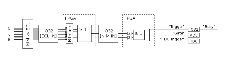
The logic starts with up to eight digital (descriminator) NIM signals being sent into a NIM -> ECL level converter. The output is then sent via a ribbon cable to the "ECL inputs" of the IO32. The eight signals are then processed in the IO32's internal FPGA. First they are sent through a bitmask, where individual channels can be ignored by writing the appropriate bits to an FPGA register. This allows individual channels to be removed from or added to the trigger logic without physically unplugging/plugging in any cables. From here, the unmasked channels are ORed to create a single "master" trigger signal, which is output via a LEMO cable from the IO32. This signal is then routed back into the IO32 via one of its NIM inputs: it is sent into either NIM input 2 or 3. These two signals (NIM in 2 and 3) are ORed internally and sent through an FPGA logic sequence to generate three output signals:
- "Trigger"
- "Gate"
- "TDC Trigger"
The "trigger" signal is routed back into the IO32, where it sets off the internal logic to identify that an event has occured. This also prompts the generation of a "busy" signal which can be used to block the generation of additional triggers while the current event is processing. The arrival time of the "trigger" signal is also stored in an internal register, and serves as the "timestamp" to identify coincidence vs. singles events (more on this later). The "gate" signal is a NIM logic pulse with a programmable width, and it is routed into the ADC(s) to serve as their common integration or peak-finding window. The "TDC trigger" signal is also a NIM logic pulse, which can be delayed by a programmable amount of time. It is routed into the TDC, where it serves as the "trigger" (this is similar to a "stop" signal - the TDC will time pulses arriving within a programmable time window proceeding the arrival of the trigger).
Data Format
MIDAS
This section gives a brief overview of the MIDAS data format and, more importantly, how it is decoded for DRAGON data analysis. This is in no way exhaustive, and for more information, the reader should consult the MIDAS documentation page. Readers who are already familiar with the MIDAS data format may wish to skip to the MIDAS Banks section where the specifics of DRAGON data are discussed. For more information on MIDAS event structure, consult https://midas.triumf.ca/MidasWiki/index.php/Event_Structure .
MIDAS files are first organized into "events". For DRAGON, each event corresponds to a single trigger of the VME system(s). The analysis code handles everything on an event-by-event basis: each event block is fully analyzed before moving onto the next one. This means that the analyzer code needs some way of obtaining the individual blocks of data that correspond to a single event. This is mostly handled using "library" functions provided as part of the MIDAS package - in other words, we let the MIDAS developers handle the details of grabbing each event's data and simply incorporate the functions they have written into our own codes.
Events are obtained in different ways depending on whether we are analyzing "online" data (data that are being generated in real time and sent to the backend analyzer via the network) or "offline" data (data stored in a MIDAS [.mid] file on disk). For online data, we use a set of routines that periodically poll the frontend computer, asking if any new events have been generated. When the frontend responds with a new event, the corresponding data are copied into a section of RAM allocated to the analysis program (often called the "event buffer"). At this point, the data now are part of the analysis program, and can be further processed using a suite of specifically designed analysis routines. For offline data, we again make use of stock MIDAS routines to extract event data into a local buffer for analysis. However, here we are not asking for events in real time; instead, we are extracting them from a file consisting of a series of events strung together. To do this, we use a set of functions that understand the detailed structure of a MIDAS file and can figure out the exact blocks of data corresponding to single events.
Once we have obtained an event and stored it in a local analysis buffer, the next step is to identify the individual packets containing data from the various VME modules. Actually, there is one important step coming before this: the individual events are placed into a local buffer (a "buffer of buffers") and, after a certain amount of time, pre-analyzed to check for coincidence matches. For more on this, see the coincidence matching section. As mentioned above, once we have a single, defined event, we need to break it down into packets or "banks" in order to analyze the data from individual VME modules. Each bank contains a header with some unique identifying information about the bank, and from there the actual bank data follow. In the header, each bank is identified by a unique 4-character string. All we have to do, then, is use library routines which search for banks keyed by their ID strings. If the corresponding bank is present within the current event, the routine will return a pointer to the memory address of the beginning of the bank, along with some other relevant information, such as the total amount of data in the event and the type of data being stored.
The actual data are simply a series of bits organized into constant-sized chunks. Each "chunk" is a unique datum (a number), corresponding to one of the C/C++ data types. Depending on how the data were written, each number could be the most basic source of information, summarizing everything there is to know about a given parameter, or it could be further sub-divided into smaller pieces of information given by the sequence of bits that make up the number within the computer. If the data are "bitpacked," then typically the code will make use of bit shifting and bit masking operators to extrack the information from the desired bits (more on this in the example below).
The only way to know how to properly handle the data is to know ahead of time how the data were written and how their relevant information is written into the various chunks of data making up a MIDAS bank. A typical analysis code will loop over all of the data in the bank, and then decide how to handle it based either on foreknowledge of the exact bank structure or on information contained in specific bits within each word.
As an example, take a slightly modified version of the code to unpack V792 ADC data:
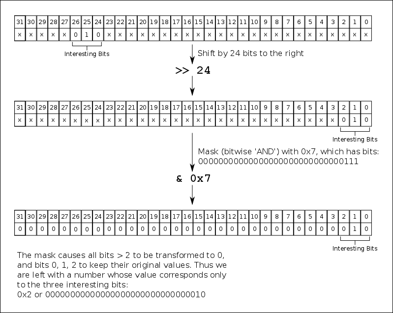
If you are unfamiliar with C/C++ bit shifting and masking, the line (*pbuffer >> 24) & 0x7 might be confusing to you. The basic idea is that you are taking the value of the 32 bits stored at the address pointed to by pbuffer (*pbuffer extracts the value) and first shifting it by 24 bits, then masking it with the value of 0x7, that is, extracting only the first three bits, which now correspond to bits 24, 25, 26 since *pbuffer has already been shifted by 24 bits to the right. Here is a figure to help visualize the process:
MIDAS Banks
The frontend codes generate four different types of events, with the following characteristics:
- "Head Event"
- Event Id: 1 (or DRAGON_HEAD_EVENT in definitions.h)
- MIDAS Equipment:
HeadVME - Trigger condition: OR of all BGO channels
- Banks:
- "VTRH": IO32 data
- "ADC0": V792 QDC data
- "TDC0": V1190 TDC data
- "TSCH": Timestamp counter data from the IO32
- "Head Scaler Event"
- Event Id: 2 (or DRAGON_HEAD_SCALER in definitions.h)
- MIDAS Equipment:
HeadScaler - Trigger condition: polled once per second
- Banks:
- "SCHD": Scaler counts (for the current read period, ~1 second)
- "SCHS": Scaler sum (since the beginning of the run)
- "SCHR": Scaler rates (counts/second for the current read period)
- "Tail Event"
- Event Id: 3 (or DRAGON_TAIL_EVENT in definitions.h)
- MIDAS Equipment:
TailVME - Trigger condition: OR of all heavy ion detectors
- Banks:
- "VTRT": IO32 data
- "TLQ0": V785 ADC data (unit 0).
- "TLQ1": V785 ADC data (unit 1).
- "TLT0": V1190 TDC data
- "TSCT": Timestamp counter data from the IO32
- "Tail Scaler Event"
- Event Id: 4 (or DRAGON_TAIL_SCALER in definitions.h)
- MIDAS Equipment:
TailScaler - Trigger condition: polled once per second
- Banks:
- "SCTD": Scaler counts (for the current read period, ~1 second)
- "SCTS": Scaler sum (since the beginning of the run)
- "SCTR": Scaler rates (counts/second for the current read period)
CAEN V792/V785 ADC
The data format of CAEN V792 charge-sensing and CAEN V785 peak-sensing ADCs is exactly the same; in fact, identical code is used to write and to analyze the data stored by each module. A single event from a V792/V785 is organized into 32-bit "longwords". A generic event looks something like this:
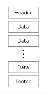
starting with a header longword, followed by a series of data longwords, and finishing with a footer longword. Each of these longwords contains multiple pieces of information given by individual series of bits within the longword. The bit structure and purpose of each type of longword is as follows:
Header
The header longwords give specific information about the module and the current event. The data are sub-divided into bits as follows:
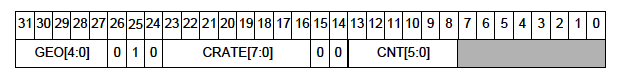
- Bits 0 - 7: Unused
- Bits 8 - 13: Identify the total number of data longwords in the event.
- Bits 14 - 15: Unused
- Bits 16 - 23: Identify the "crate number" of the present module (ignored for DRAGON experiments).
- Bits 24 - 26: Uniquely identify the longword as a header, that is, all headers have the sequence 0 1 0 for these bits.
- Bits 27 - 31: Identify the "geo address" of the present module (ignored for DRAGON experiments).
Data
The data longwords tell the actual measurement value of a specific channel, that is, they tell what the integrated charge or maximum height of the signal going into a single channel is. Data longwords are arranged as follows:
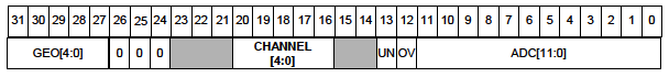
- Bits 0 - 11: Encode the measurement value for the channel in question. Note that since this is an 12-bit number, the measurement values can be within the range [0, 4095] (or [0x0, 0xfff]).
- Bit 12: Single bit telling if the channel in question was in an overflow condition (signal larger than the maximum). '1' corresponds to a channel that is in overflow, '0' to one not in overflow.
- Bit 13: Same as bit 12, except it tells if the channel is in an _under_flow condition (below a certain threshold).
- Bits 14 - 15: Unused.
- Bits 16 - 20: Encode the number of the channel in question, i.e. if these bits evaluate to 5, we are reading input channel five, and so on.
- Bits 21 - 23: Unused.
- Bits 24 - 26: Uniquely identify the longword as a "data" word: all data words have the sequence 0 0 0 for these bits.
- Bits 27 - 31: Copy of the "geo" address from the header.
Footer
The main purpose of footer lngwords is to provide a counter for the total number of events received during a run.
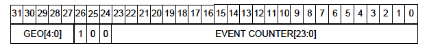
- Bits 0 - 23: Event counter, increments automatically every time a new event is read.
- Bits 24 - 26: Ideitify this longword as a footer; all footers have the sequence 0 0 1 for these bits.
- Bits 27 - 31: Copy of the "geo" address.
Finally, in addition to the types mentioned above, a longword can also be an invalid word, which is IDed by 0 0 1 for bits 24 - 26. An invalid word typically signifies some sort of error condition within the ADC.
CAEN V1190 TDC
The structure of a V1190 TDC event is somewhat similar to that of a V792/V785 ADC: each event consists of a series of longwords, with the general structure of [Header], [Data], [Data], ..., [Data], [Footer]. In addition, there is also a "global" header attached to each event. Unlike the V792, we do not necessairily have only a single data longword per channel; this is because the V1190 is a "multi-hit" device, that is, it is capable of registering multiple timing measurements if more than one pulse goes into a given channel during recording of an event. Additionally, the user may set the TDC to record the time of both the front and the back of a given pulse, and each of these will count as a different "hit" on the channel.
Below are the bit packed structures of the various types of longwords that can be read from a V1190 TDC. Note that the V1190 is a rather complex device and can run in varying operating modes. The documentation below is only relevant in the "trigger matching" mode, which is how DRAGON operates. For information about other running options, consult the manual (available online from the CAEN website).
Global Header
The global header contains an event counter and some other common information about the module.
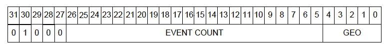
- Bits 0 - 4: "Geo" address (unused for DRAGON).
- Bits 5 - 26: Event counter.
- Bits 27 - 31: Identify the longword in question as a global header with the unique sequence of 0 0 0 1 0 for these bits.
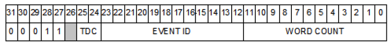
TDC Header
The (optional) TDC header contains information about a apecific TDC trigger.
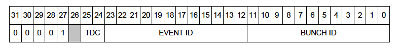
- Bits 0 - 11: Encode the bunch id of the trigger.
- Bits 12 - 23: Encode the event ID.
- Bits 24 - 25: TDC code (unused for DRAGON).
- Bit 26: Unused.
- Bits 27 - 31: Identify the longword in question as a TDC header by having the sequence 1 0 0 0 0.
Measurement
A measurement longword contains the information of a single timing measurement made by the device.
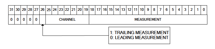
- Bits 0 - 19: Encode the measurement value. As an 19-bit number, this allows measurements in the range
[0, 524287](or[0x0, 0x7ffff]). - Bits 19 - 25: Encode the channel number of the measurement in question.
- Bit 26: Tells whether the measurement in question is a trailing-edge measurement ('1') or a leading-edge measurement ('0').
- Bits 27 - 31: Identify the longword in question as a measurement by having the sequence 0 0 0 0 0.
TDC Trailer
The (optional) TDC Trailer provides some additional information about a TDC trigger.
- Bits 0 - 11: Count of the number of words read from the trigger.
- Bits 12 - 23: ID code of the trigger.
- Bits 24 - 25: TDC code (unused for DRAGON).
- Bit 26: Unused.
- Bits 27 - 31: Identify the longword in question as a TDC trailer by having the sequence 1 1 0 0 0.
Global Trailer
The global trailer contains some information that is common to all events.
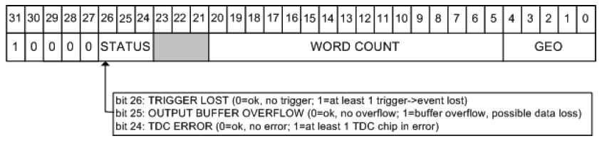
- Bits 0 - 4: "Geo" address of the module (unused in DRAGON).
- Bits 5 - 20: Number of words currently read.
- Bits 21 - 23: Unused.
- Bits 24 - 26: Encodes the status of the current event. If all three bits are zero, then we are in a "no error" condition. For the various "error" conditions and the bits that signal them, consult the figure.
- Bits 27 - 31: Identify the current longword as a global trailer via the sequence 0 0 0 0 1.
Error
This type of longword is only present if the TDC is in an error condition.
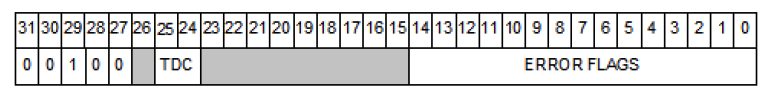
- Bits 0 - 14: Encode the error status. Each bit that is set to '1' signifies a unique error condition:
- [0]: Hit lost in group 0 from read-out FIFO overflow.
- [1]: Hit lost in group 0 from L1 buffer overflow
- [2]: Hit error have been detected in group 0.
- [3]: Hit lost in group 1 from read-out FIFO overflow.
- [4]: Hit lost in group 1 from L1 buffer overflow
- [5]: Hit error have been detected in group 1.
- [6]: Hit data lost in group 2 from read-out FIFO overflow.
- [7]: Hit lost in group 2 from L1 buffer overflow
- [8]: Hit error have been detected in group 2.
- [9]: Hit lost in group 3 from read-out FIFO overflow.
- [10]: Hit lost in group 3 from L1 buffer overflow
- [11]: Hit error have been detected in group 3.
- [12]: Hits rejected because of programmed event size limit
- [13]: Event lost (trigger FIFO overflow).
- [14]: Internal fatal chip error has been detected.
- Bits 15 - 23: Unused.
- Bits 24 - 25: TDC code (unused for DRAGON).
- Bit 26: Unused.
- Bits 27 - 31: Identify the current longword as an error word via the sequence 0 0 1 0 0.
IO32 FPGA/Control Board
Data from the IO32 FPGA/control board are written into two separate MIDAS banks. The first bank contains information about the trigger conditions generating the present event. It consists of nine 32-bit longwords, and each longword, save for one, corresponds to a single piece of information about the trigger (i.e. no sub dividing into bits as with the CAEN modules). The nine longwords read from the trigger bank are as follows:
- Header and version number of the IO32.
- Number of triggers (starting with zero) since the beginning of the run.
- Timestamp marking the arrival of the trigger signal.
- Timestamp marking when the data readout began.
- Timestamp marking when the data readout ended.
- Trigger latency: the difference in timestamps between the trigger and the start of the readout.
- Readout elapsed time: the difference in timestamps between the end of the readout and the start of the readout.
- Busy elapsed time: the difference in timestamps between the end of the readout and the trigger.
- Trigger latch value: This is the only bitpacked value in the IO32 trigger bank. The first eight bits in the longword signify which of the eight input channels generated the trigger. Whichever bit is true is the channel making the trigger. For example, a value of 0x4 [ bits: 00000000000000000000000000000100 ] means that input 3 generated the trigger.
The other bank consisting of IO32 data is the timestamp counter (TSC) bank. This bank contains timestamp information for both the event trigger and other programmable channels (such as the "cross" trigger, or the trigger of the other DAQ, if it is present). It is here that we look to identify which events are singles events and which are coincidences. The actual TSC data are stored in a FIFO (first in, first out) with a maximum depth set by firmware limitations. Any pulses arriving beyond the limits of the FIFO are ignored.
The TSC banks are arranged as follows (all 32-bit unsigned integers).
- Version number (firmware revision tag).
- Currently ignored other than a check that the version numbner is a known one.
- Currently ignored other than a check that the version numbner is a known one.
- Bank timestamp (time at which the TSC bank was composed).
- Currently ignored.
- Currently ignored.
- TSC routing bits (sets TSC signal routing for the frontend)
- Ignored for analysis.
- Ignored for analysis.
- TSC control
- Contains the following bitpacked information:
- Bits 13..0 - Number of TSC words in the FIFO
- Bit 14 - FIFO overflow marker
- Bits 21..15 - Upper 8 bits common to each TSC in the FIFO.
- Contains the following bitpacked information:
- Upper bits rollover
- Firmware limits each TSC measurement to 38 bits, which rolls over in ~3.8 hours. Runs could occasionally go longer than this, so we manually count the number of rollovers in the upper 8 bits in the frontend code and write it here.
- Firmware limits each TSC measurement to 38 bits, which rolls over in ~3.8 hours. Runs could occasionally go longer than this, so we manually count the number of rollovers in the upper 8 bits in the frontend code and write it here.
- FIFO (depth given by TSC control as noted above)
- Each entry is bitpacked as follows:
- Bits 0..29 - Lower 30 bits of the timestamp entry (combine with upper 8 bits plus upper bits rollover marker)
- Bits 30..31 - Channel marker (0,1,2,3) for this TSC measurement
- Each entry is bitpacked as follows:
- Overflow marker: additional word
== 0xFFFFFFFFis written if the TSC is in an overflow condition.- Currently ignored because TSC control gives the same information.
Coincidence Matching
An important topic related to the TSC bank is the method used to identify singles and coincidence events. As analysis of real-time, online data is quite important for DRAGON experiments, we need a method that is able to handle potential coincident head and tail events arriving at the backend at relatively different times. Since, as mentioned, MIDAS buffers events in the frontend before transferring to the backend via the network, events from each side are received in blocks. Potantially, coincident events could be quite far separated in terms of "event number" arriving at the backend.
The method used to match coincidence and singles events is to buffer every incoming event in a queue, sorted by their trigger time values. In practice, this is done using a C++ standard library multiset, as this container was shown to be the most efficient way in which to order events by their trigger time value. Whenever a new event is placed in the queue, the code checks its current "length" in time, that is, it checks the time difference between the beginning of the queue (the earliest event) and the end of the queue (the latest event). If this time difference is greater than a certain value (user programmable), then the code searches for timestamp matches between the earliest event and all other events in the queue. Note that a "match" does not necessairily mean that the trigger times are exactly the same, as this would imply that the heavy ion and γ-ray were detected at exactly the same time, which is impossible for a real coincidence since the heavy ion must travel for a finite amount of time (~3 μs). Thus, we define a "match" as two triggers whose time difference is within a programmable time window. Typically, this window is made significantly larger than the time difference of a true coincidence (~10 μs), and further refinements can be made later by applying gates to the data.
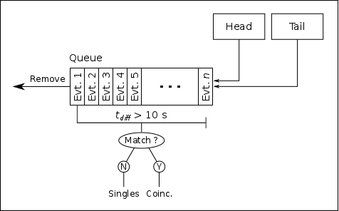
If a match is found, then the two events are analyzed as coincidences, and the earliest event is removed from the queue. If no match is found, the earliest event is analyzed as a singles event and then removed from the queue. As long as the maximum time difference is set large enough to cover any "spread" in the arrival times, this algorithm should guarantee that every coincidence is flagged as such.
Installation
This section gives an overwiew of how to obtain and install the latest version of the DRAGON data analysis package.
- Note
- These instructions assume that you will install the dragon analyzer package in
~/packages/dragon. If not, it will be necessary to alter the paths given below accordingly.
Dependencies
For the "core" functionality, all that you will need is a working C++ compiler; there is no dependence on any third-party libraries. However, you will likely want to make use of the analysis package in ROOT, in which case you will need a fairly recent installation of ROOT on your system. For instructions on installing ROOT, go here. It is suggested that you install a relatively recent version of ROOT (say, ≥ 5.30) to ensure combatibilty between the ROOT release and the package code. You will also need to be sure that the $ROOTSYS environment variable is set and that $ROOTSYS/bin is in your search path. This is typically accomplished by sourcing the thisroot.sh or thisroot.csh script in $ROOTSYS/bin from your startup script (e.g. - ~/.bashrc).
- Attention
- Ubuntu users: compiling the DRAGON analyzer package evidently requires
clang(sudo apt-get install clang clang++).
- Note
- The DRAGON analyzer package is now compatible with ROOT6, but ROOT6 functionality should be considered beta until it has been tested more rigorously. Please report bugs to dconnolly@triumf.ca or file an issue here.
The optional rootbeer or rootana extensions each require ROOT to be installed (and, of course, the rootana and/or rootbeer packages themselves). To look at online data, you will need MIDAS installed, and, if using the rootana system, roody is required for online histogram viewing.
Download and Compile
One may obtain the analysis package from the git repository as follows:
mkdir -p ~/packages/dragon
cd ~/packages/dragon
git clone https://github.com/DRAGON-Collaboration/analyzer
cd analyzer
If you do not have git installed or prefer to download a tarball, then visit https://github.com/DRAGON-Collaboration/analyzer, click on the releases link and select the latest release (or an earlier one if you have reason to do so). Click on either the "zip" or the "tar.gz" link to download a zip file or a tarball containing the code.
Once the package is obtained, it is necessary to run a configure script in order to set the appropriate environment variables before compiling. To see a list of options, type:
./configure --help
In most cases, one may simply run
./configure
At this point, compilation should be as simple as typing make. If not, please let me know, and we can try to fix the problem permanently so others do not run into it.
Compilation creates a shared library lib/libDragon.so (and lib/libDragon.so.dSYM if installed on a Mac) as well as an executable bin/mid2root. The executable converts MIDAS files to ROOT trees. The library can be loaded into an interactive ROOT session by issuing the following commands:
root[] .include ~/packages/dragon/analyzer/src
root[] gSystem->Load("~/packages/dragon/analyzer/lib/libDragon.so");
It is strongly suggested that you add the appropriate lines to your root logon script if you have one. If you do not, the proper way to set up your root environment is to create a file entitled rootlogon.C in a sensible place (such as ~/packages/root/macros) and include the following lines in it:
Then create the file ${HOME}/.rootrc (if it doesn't already exist) and include the following line in it:
Examples of rootlogon.C and .rootrc are given in the script directory. This will give you access to all of the dragon classes and functions in the software package from within a ROOT session or macro.
If you are using git and want to stay on top of new releases, just do:
git pull master --tags
from within the repository directory (~/packages/dragon/analyzer). This gets you all of the new code since your last pull (or the initial clone). Note that we have started using a versioning system than goes as such: vMAJOR.MINOR.PATCH, where a MAJOR version change indicates a new set of non backwards compatible changes. MINOR indicates a feature addition that is still backwards compatible, and PATCH indicates a bugfix or other small change that is backwards compatible.
Python Extension
- Note
- No one has kept up with maintaining the python extension in quite a while and it is not a priority. Really, it was just a "fun" project to play around with using
Py++andBoost.Python, but it should not take too much to get it running again if anyone is interested...
If you wish to compile or use the optional (and somewhat experimental) python extension, you will first need to install the Boost.Python library. For information on this, see: http://www.boost.org/doc/libs/1_66_0/libs/python/doc/html/index.html
The python libraries rely on code generated by Py++, which parses the source files and generates code to be compiled into the python libraries. It should not be necessary to generate the source code yourself using Py++, as long as the repository is kept up-to-date; however,if you make changes to the dragon analyzer sources, re-generation of the Py++ sources will be necessary in order to safely use the python libraries.
To compile the python extension, simply cd into the py++ directory and type make, after having compiled the core dragon library. To be able to use the extensions from any directory, add the following to your bash startup script (e.g. - ~/.bashrc):
and re-start your bash session or re-source the startup script. Now from a python session or script, you can load the generated modules:
You can use the python 'help' function (help dragon, etc) to see the classes and functions available in each module.
For Users
Rootana Online Analyzer
This package includes a library to interface the DRAGON analysis codes with MIDAS's rootana system, which allows visualization of online and offline data in histograms. If you are familiar with the "old" DRAGON analyzer, this is essentially the same thing, but with a few added features. To use this analyzer, simply compile with the "USE_ROOTANA" option set to "YES" in the Makefile (of course, for this to work, you will need to have the corresponding MIDAS packages installed on your system). Then run the anaDragon executable, either from a shell or by starting it on the MIDAS status page. To see a list of command line option flags, run with the -h flag. To view histograms, you will need to run the 'roody' executable, which should be available on your system if you have MIDAS installed.
As mentioned, there are a couple feature additions since the previous version of the DRAGON analyzer. The main one is the ability to define histograms and cuts at run-time instead of compile time. The hope is that this will allow for easy and quick changes to be made to the available visualization, even for users who are completely inexperienced with C++.
Histograms are created at run-time (anaDragon program start) by parsing a text file that contains histogram definitions. By default, histograms are created from the file $DRAGONSYS/histos.dat, where $DRAGONSYS is the location of the DRAGON analyzer package. However, you can alternatively specify a different histogram definition file by invoking the -histos flag at program start:
./anaDragon -histos my_histograms.dat
Note that the default histogram file (or the one specified with the -histos flag, creates histograms that are available both online and offline, that is, they are viewable online using the roody interface, and they are also saved to a .root file at the end of the run. It is also possible to specify a separate set of histograms for online viewing only. To do this, invoke the histos0 flag:
./anaDragon -histos0 histograms_i_only_care_to_see_online.dat
Now that you know how to specify what file to read the histogram definitions from, you should probably also know how to write said file. The basic way in which the files are parsed is by using a set of "key" codes that tell the parser to look in the lines below for the appropriate information for defining the corresponding ROOT object. The "keys" available are as follows:
- DIR: Create a directory.
The succeeding line should contain the full path of the directory as plain text.
For example:This would create a new directory "histos", with "gamma" as a sub-directory. Note that if you later doDIR:histos/gammathe "histos" directory would not be re-created; instead, "hion" would be added as a new sub-directory. When you specify a directory, any histogram definitions succeeding it will be members of that directory, until another directory line is encountered. If any histograms are defined before the first "DIR:" command, they will belong to the "top level" directory (e.g. in aDIR:histos/hionTFile, their owning directory will be theTFileitself).
- TH1D: Create a 1d histogram.
Should be succeeded by two lines:
1) the argument to aTH1Dconstructor
2) the parameter to display in the histogram.
Example:(note that the indentations are only for readability, not required). This creates a histogram with name "`bgo_e0`", title "Bgo energy, channel 0 [singles]", and ranging from 0 to 4096 with 256 bins. The parameter to be displayed in the histogram would beTH1D:("bgo_e0", "Bgo energy, channel 0 [singles]", 256, 0, 4096)rootana::gHead.bgo.ecal[0]rootana::gHead.bgo.ecal[0].
- TH2D: Create a 2d histogram.
Succeeding lines are in the same spirit as the 1D case, except a third line is added to specify the y-axis parameter.
Example:Creates a histogram ofTH2D:("bgo_e1_e0", "Bgo energy 1 vs. 0 [coinc]", 256, 0, 4096, 256, 0, 4096)rootana::gCoinc.head.bgo.ecal[1]rootana::gCoinc.head.bgo.ecal[0]rootana::gCoinc.head.bgo.ecal[1][x-axis] vs.rootana::gCoinc.head.bgo.ecal[0][y-axis].
- TH3D Create a 3d histogram.
Following the same pattern as 1d and 2d - add a third line to specify the z-axis parameter.
- SCALER: Create a "scaler" histogram, that is a 1d histogram whose x-axis represents event number and y-axis represents number of counts (basically, abuse histogram to make it into a bar chart).
The lines following a "SCALER:" command are:
1) Constructor for a 1D histogram, which defines the x-axis (event) range and binning. Typically you want to start at zero and bin with 1 bin per channel. Note that the histogram will automatically extend itself if the number of events exceeds the x-axis range.
2) The scaler parameter you want to histogram.
Example:SCALER:("rate_ch0", "Rate of scaler channel 0", 5000, 0, 5000);rootana::gHeadScaler.rate[0]
- SUMMARY: Create a "summary" histogram, that is a histogram which displays information on multiple channels at once, like this:
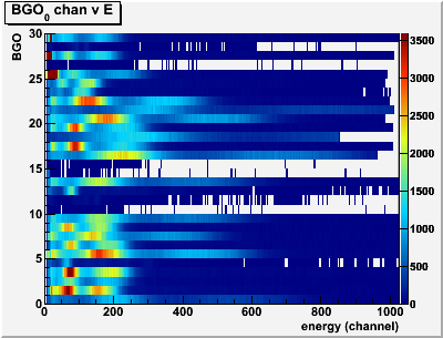
Note that summary histograms are currently only available for arrays, that is, where each y-axis bin corresponds to a different array index. If you need to display summary information for parameters not contained in an array, you will have to define the histogram manually in C++. However, in nearly all cases where summary information might be desired, the parameters are already contained in an array anyway.
The lines following a "SUMMARY:" command are:
1) Constructor for a 1d histogram; this will define the x-axis binning and set the histogram name/title;
2) The name of an array that you want to display in the histogram;
3) The number of y-axis bins (should be equal to the length of the array).
Example:This would create a summary histogram of the 30 BGO detector energies contained in theSUMMARY:("bgo_q", "Bgo energies [singles]", 256, 0, 4096)rootana::gHead.bgo.ecal30rootana::gHead.bgo.ecalarray (bgo.ecal[0]→bgo.ecal[29]).
- CUT: Defines a cut.
This defines a "cut" or "gate" condition that will be applied to the histogram defined directly before it. The cut condition is specified as a logical condition consisting of rootana::Cut derived classes. For more information on how to define a cut, see the code documentation of the Cut.hxx source file and links therein. As a simple example:will create the "bgo_e0" histogram displayingTH1D:("bgo_e0", "Bgo energy, ch 0 [singles]", 256, 0, 4096)rootana::gHead.bgo.ecal[0]CUT:Less(gHead.bgo.ecal[0], 2000) && Greater(gHead.bgo.ecal[0], 100)bgo.ecal[0], with the condition thatbgo.ecal[0]be greater than 100 and less than 2000.
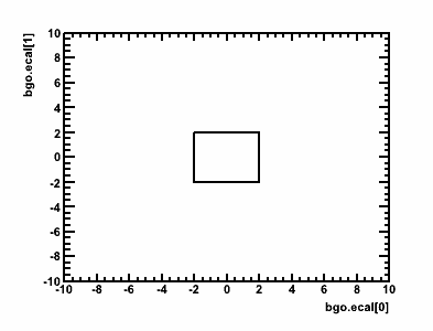
Note that you can also create/use 2d polygon cuts, either by specifying the parameters and (closed) polygon points:This would create the following cut:CUT:Cut2D(gHead.bgo.q[0], gHead.bgo.q[1], -2,-2, -2,2, 2,2, 2,-2, -2,-2)
It is also possible to pre-define and then re-use graphical cuts using the "CMD:" option (see next).
- CMD: Evaluates a series of commands in CINT.
The succeeding lines are a series of C++ statements to be evaluated literally in the CINT interpreter, closed by a line containing only "END". Any objects created within these statements will become available for use in future commands throughout the definition file. Note that each file should only contain one "CMD:" statement (if it contains any), and that it should be the first "active" code within the file. As an example, we could use "CMD:" to define a graphical cut:This cut is then available in future statements; for example to create a Cut2D object to be applied to a histogramCMD:TCutG cutg("cutTest",7);cutg.SetVarX("");cutg.SetVarY("");cutg.SetTitle("Graph");cutg.SetFillColor(1);cutg.SetPoint(0,37.8544,70.113);cutg.SetPoint(1,25.5939,41.5819);cutg.SetPoint(2,54.9042,28.0226);cutg.SetPoint(3,83.0651,35.3672);cutg.SetPoint(4,81.5326,53.1638);cutg.SetPoint(5,59.3103,79.1525);cutg.SetPoint(6,37.8544,70.113);ENDThe above example would apply the graphical cut "cutg" defined in the "CMD:" statement to the "bgo_ecal" histogram.SUMMARY:("bgo_ecal", "Bgo energies [singles]", 256, 0, 4096)rootana::gHead.bgo.ecal30CUT:Cut2D(gHead.bgo.ecal[0], gHead.bgo.ecal[1], cutg)
With combinations of the above commands, you should hopefully be able to define any histogram-related objects you will need in the online analyzer without ever having to touch the source code. A few more notes about histogram definition files:
- There are five global instances of "top-level" classes which encapsulate all of the relevant data in the experiment. Each class corresponds to a different event type, and is mapped to a different ROOT tree in the output file. As you may have noticed in the examples, these will need to prefix any parameters to be displayed in histograms. They are:
rootana::gHead- "Head" (gamma) singles eventrootana::gTail- "Tail" (heavy-ion( singles eventrootana::gCoinc- Coincidence eventrootana::gHeadScaler- "Head" (gamma) scaler eventrootana::gTailScaler- "Tail" (heavy-ion) scaler event
- White-space is ignored, though good indention improves readability immensely.
- The
#character denotes a comment, all characters on the same line coming after a#are ignored:# IGNORE THIS HEADER STATEMENT #TH1D: #Ignore this descriptive comment also... - The run-time parsing is done using CINT via the
gROOT->ProcessLine()andgROOT->ProcessLineFast()commands. These have very little native error handling. Some support has been added in the DRAGON analyzer to "gracefully" handle common errors when detectable; for example, skipping the current definition and moving onto others, but alerting the user. If you find a case where you feel the error handling could be improved (in particular, where a mistake in the script file causes a crash or un-reported failure), do not hesitate to alert the developers.
Once started, the online analyzer simply runs in the background to receive, match, and analyze events coming from the two separate front-ends. The analyzed data are then summarized in the histograms requested by the user as outlined in the proceeding paragraphs. As mentioned, roody can be used to visualize the histograms as data is coming in. To start roody, you will need to specify the host and port of the histogram server. Usually this means, the following:
roody -Plocalhost:9091
if running locally from the back-end host, or
roody -Pdaenerys.triumf.ca:9091
if running remotely. Roody is a graphical program, and as such its use is fairly intuitive. When you start the program, you should see a graphical outline of the histograms and directory structure you created in your hist definitions file that looks something like this:
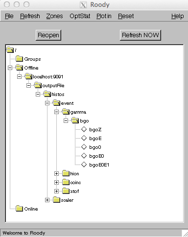
Simply double click on a histogram icon, and a ROOT canvas will be created showing the histogram. You can play around with the menu bars to explore other options, such as canvas refresh rate and canvas configuration.
For Developers
This section just gives a brief overview behind the package's design and some suggestions for future maintainers/developers. For detailed documentation, see the related Doxygen documentation linked from the top of this page.
Design
In writing this code, I have tried to adhere to a few design principles. I will give a brief listing here in hopes that future developers (or users) of the code can better understand what is going on and the reasoning behind it. In the future (barring a major re-write), I think it will be beneficial to follow a similar design pattern for modifications and updates to the code, if for no other reason than to keep a sense of uniformity which will hopefully facilitate understanding of the code.
- Separate the handling of "raw" data from that of abstract experiment parameters.
By this I mean separating the "raw" tasks of reading data directly from VME modules from that of organizing the data into parameters which represent more abstract experimental quantities. As a simple example, separate the "raw" task of reading the conversion value of QDC channel 27 from the "abstract" task of realizing that this value corresponds to the energy deposited in BGO detector number 27. The hope is that by de-coupling the two different types of operations, we will gain greater flexibility and re-usability of the code.
To accomplish this, there are separate "vme" classes (under the vme namespace) which handle the unpacking of raw vme data. Each vme class contains data fields to store its respective measurements. For example, see the documentation ofvme::V792, which represents a CAEN V792 QDC module.
Store abstract experiment parameters in classes which logically correspond to the separate pieces of a DRAGON experiment.
The basic idea is that we want to take the important data captured during a DRAGON event and break it down into a tree-like structure. In general, each "branch" of the tree corresponds to a different detector within the DRAGON system, and the various "leaves" correspond to quantities measured by that detector. For example, see the dragon::Coinc documentation and the "Attribute" links therein.
Taking this approach allows a couple of practical advantages beyond code organization and maintenance. The main one is that we can use ROOT's dictionary facility to createTTrees whith branches defined by the structure of our classes. For example we can just do:TTree tcoinc("tcoinc","Coincidence event");tcoinc.Branch("coinc","dragon::Coinc",&coinc);After just a few lines of code, we now have the ability to access any parameter in a DRAGON coincidence event through the 'tcoinc' tree:
tcoinc.Draw("coinc.head.bgo.ecal[0]>>hst_e0(400,0,4000)"); // Draws BGO energy, channel 0tcoinc.Draw("coinc.tail.mcp.tac>>hst_tac(200,0,2000)"); // Draws MCP TOFIn writing the DRAGON classes, I have not used any sort of inheritance, as there is really no compelling reason to do so (in particular, we have no need for dynamic polymorphism). I have, however, tried to maintain a uniform interface for each of the classes. For example, each detector class has the following three methods:
read_data()- Takes raw data from vme module classes and maps it into the class's internal data structures.calculate()- Performs any necessary calculations on the raw data; for example, this could include things such as pedestal subtraction, channel calibration, or calculation of quantities which depend on multiple signals.reset()- Resets all of the class's internal data to a "default" throwaway value; in most cases this will be equivalent todragon::NO_DATA.
Developing with a common interface, aside from being "neater" allows for some practical advantages, such as using template "helper" functions to bundle routines used for a variety of different classes. For example:template <class T>{detector.reset();detector.read_data(adc, tdc);detector.calculate();}void handle_all_events(){handle_event(mcp, adc, tdc); // mcp is an instance of dragon::Mcphandle_event(ic, adc, tdc); // ic is an instance of dragon::IonChamber// ... etc ... //}Another feature that I have adhered to is to allow class data members to be public. Although this goes against canonical object oriented good principles, I think the advantages outweight the disadvantages. This is particularly true if we are working in CINT to analyze data.1 For example, with public data, it's trivial to loop over a tree, calculate some new parameter and display it in a histogram. For example, say I want to plot the square of MCP time-of-flight in cases where it is nonzero:
// Assume prior existance of a TTree 't' containing heavy-ion datadragon::Tail tail;void* tailAddr = &tail;t->SetBranchAddress("tail", &tailAddr);TH1D hst("hst", "MCP Tof **2", 100, 0, 10000);for(Long64_t event = 0; event < t->GetEntries(); ++event) {t->GetEntry(event);hst.Fill(pow(tail.map.tac, 2));}}hst->Draw();However, despite the usefulness of public data for scripting use, it is still a good idea to design the source code as if the data were private. This reduces the coupling between the various classes, and as a result making a small change to the structure of one class (or module) is guaranteed not to affect the others. To enforce this, I have defined a macro
PRIVATEwhich can be set to be equal to eitherprivateorpublicin the Makefile and defined all of the class data members under this token.class SomeDetector {PRIVATE:double some_parameter;// etc. //};When developing the source code, one should make sure it will compile with PRIVATE=private - to enforce good class design. Then when set up for "production" mode, switch over to PRIVATE=public to allow direct variable access in CINT (and in the python modules, if used).
- Add a layer of abstraction for commonly performed routines.
For example, to read raw QDC data into thedragon::Bgoclass, we could do:
but instead we prefer to do the following, using utils::channel_map() to do the actual mapping.{}}The main motivation for this is to concentrate the majority of the "heavy lifting" used in various calculations into one place. This helps to reduce the occurrence of bugs due to re-writing of similar code, and if bugs are found to facilitate easier fixes. Most of the "heavy lifting" is done in free functions contained in the{}dragon::utilsnamespace, or using standard library algorithms.
Coding Conventions
Finally, there are a few stylistic issues to address. Much of this is just preference, but it would be nice to keep consistency in future code.
- Make use of namespaces to logically group related classes together. For example, all classes representing vme modules are under the vme namespace, all classes representing dragon detectors or collections of detectors are under the
dragonnamespace, all midas-related stuff under themidasnamesapce and so on. Source files belonging to a common namespace are grouped into the same subdirectory withinsrc/. - Class names generally start with a capitol letter and use "CamelCase" when consisting of multiple words. Acronyms are not treated any differently, to avoid confusion; for example
class Dsssdnotclass DSSSD. - Class methods and free functions are all "CamelCase" (including acronyms) (
SomeMethodorSomeFunctionorSomeMthd). - Brackets: for everything except function definitions, keep the opening bracket on the same line and the trailing bracket on a new line:
namespace dragon {class Bgo {public:void calculate();// ... //};} // namespace dragonvoid dragon::Bgo::calculate(){// ... //}// ... //} - In any class that might be parsed into a tree structure using rootcint, class members are all lowercase, should be descriptive yet brief when parsing classes into a tree structure, and should not use any form of Hungarian notation (as it will conflict with the "nicely descriptive" requirement). This has a practical advantage when we let ROOT parse our classes into a
TTree: the brach names make sense and are logical. I would much rather type:
thant->Draw("head.bgo.ecal[0]");
For classes that are not intended to be madet->Draw("gHead.fBgo.fEnergy[0]"); // (following the ROOT / Taligent convention)TTreebranches, the ROOT/Taligent hungarian notation can be quite nice, however.
- Whenever appropriate, prefer arrays to separate variables. For example, BGO energies are defined as
instead ofdouble ecal[MAX_CHANNELS];This has a number of practical advantages, such as allowing for loops and std::algorithms to handle the data, and in general it makes life much easier in later analyses as well. It also avoids any issues about whether to start counting at one or zero, since arrays always start from zero.double ecal0;double ecal1;// ... //double ecal29;
Documentation
Given the fast turnover rate of developers and the common requirement for "everyday" users (whose level of expertise in the source language ranges from beginner to expert) to understand and modify source code, maintaining quality code documentation is essential for a physics software package to stay maintainable.
As you may have noticed, the present source code has been extensively documented using Doxygen. I do not claim that the present documentation is perfect by any means, but I hope it is at least a large step in the right direction. If you happen to extend or modify the code base, please carefully document anything that you do. If you are not familiar with Doxygen, it is quite intuitive and quick to learn - just follow the example of existing code and/or refer to the Doxygen manual.
Footnotes
1Actually, because the dictionary file generated by rootcint uses the #define private public trick to gain access to your class's internals, if you don't make all of your class data public you actually end up generating code that is not within the C++ standard and, in theory at least, can lead to undefined behavior! See, for example, this link for more on this subject. So, if you want to be as standards compliant as possible, you will have to make all of your class members public.