For Users

Rootana Online Analyzer

This package includes a library to interface the DRAGON analysis codes with MIDAS’s rootana system, which allows visualization of online and offline data in histograms. If you are familiar with the “old” DRAGON analyzer, this is essentially the same thing, but with a few added features. To use this analyzer, simply compile with the “USE_ROOTANA” option set to “YES” in the Makefile (of course, for this to work, you will need to have the corresponding MIDAS packages installed on your system). Then run the anaDragon executable, either from a shell or by starting it on the MIDAS status page. To see a list of command line option flags, run with the -h flag. To view histograms, you will need to run the ‘roody’ executable, which should be available on your system if you have MIDAS installed.

As mentioned, there are a couple feature additions since the previous version of the DRAGON analyzer. The main one is the ability to define histograms and cuts at run-time instead of compile time. The hope is that this will allow for easy and quick changes to be made to the available visualization, even for users who are completely inexperienced with C++.

Histograms are created at run-time (anaDragon program start) by parsing a text file that contains histogram definitions. By default, histograms are created from the file $DRAGONSYS/histos.dat, where $DRAGONSYS is the location of the DRAGON analyzer package. However, you can alternatively specify a different histogram definition file by invoking the -histos flag at program start:

./anaDragon -histos my_histograms.dat

Note that the default histogram file (or the one specified with the -histos flag, creates histograms that are available both online and offline, that is, they are viewable online using the roody interface, and they are also saved to a .root file at the end of the run. It is also possible to specify a separate set of histograms for online viewing only. To do this, invoke the histos0 flag:

./anaDragon -histos0 histograms_i_only_care_to_see_online.dat

Now that you know how to specify what file to read the histogram definitions from, you should probably also know how to write said file. The basic way in which the files are parsed is by using a set of “key” codes that tell the parser to look in the lines below for the appropriate information for defining the corresponding ROOT object. The “keys” available are as follows:

1. DIR: Create a directory. The succeeding line should contain the full path of the directory as plain text. For example:

DIR:
    histos/gamma

This would create a new directory “histos”, with “gamma” as a sub-directory. Note that if you later do

  DIR:
    histos/hion

the “histos” directory would not be re-created; instead, “hion” would be added as a new sub-directory. When you specify a directory, any histogram definitions succeeding it will be members of that directory, until another directory line is encountered. If any histograms are defined before the first “DIR:” command, they will belong to the “top level” directory (e.g. in a TFile, their owning directory will be the TFile itself).

1. TH1D: Create a 1d histogram. Should be succeeded by two lines:
2. the argument to a TH1D constructor
3. the parameter to display in the histogram. Example:

  TH1D:
    ("bgo_e0", "Bgo energy, channel 0 [singles]", 256, 0, 4096)
    rootana::gHead.bgo.ecal[0]

(note that the indentations are only for readability, not required). This creates a histogram with name “bgo_e0”, title “Bgo energy, channel 0 [singles]”, and ranging from 0 to 4096 with 256 bins. The parameter to be displayed in the histogram would be rootana::gHead.bgo.ecal[0].

1. TH2D: Create a 2d histogram.

Succeeding lines are in the same spirit as the 1D case, except a third line is added to specify the y-axis parameter.

Example:

  TH2D:
    ("bgo_e1_e0", "Bgo energy 1 vs. 0 [coinc]", 256, 0, 4096, 256, 0, 4096)
    rootana::gCoinc.head.bgo.ecal[1]
    rootana::gCoinc.head.bgo.ecal[0]

Creates a histogram of rootana::gCoinc.head.bgo.ecal[1] [x-axis] vs. rootana::gCoinc.head.bgo.ecal[0] [y-axis].

1. TH3D Create a 3d histogram.

Following the same pattern as 1d and 2d - add a third line to specify the z-axis parameter.

1. SCALER: Create a “scaler” histogram, that is a 1d histogram whose x-axis represents event number and y-axis represents number of counts (basically, abuse histogram to make it into a bar chart).

The lines following a “SCALER:” command are:

1. Constructor for a 1D histogram, which defines the x-axis (event) range and binning. Typically you want to start at zero and bin with 1 bin per channel. Note that the histogram will automatically extend itself if the number of events exceeds the x-axis range.
2. The scaler parameter you want to histogram.

Example:

  SCALER:
    ("rate_ch0", "Rate of scaler channel 0", 5000, 0, 5000);
    rootana::gHeadScaler.rate[0]

1. SUMMARY: Create a “summary” histogram, that is a histogram which displays information on multiple channels at once, like this:

Note that summary histograms are currently only available for arrays, that is, where each y-axis bin corresponds to a different array index. If you need to display summary information for parameters not contained in an array, you will have to define the histogram manually in C++. However, in nearly all cases where summary information might be desired, the parameters are already contained in an array anyway.

The lines following a “SUMMARY:” command are:

1. Constructor for a 1d histogram; this will define the x-axis binning and set the histogram name/title;
2. The name of an array that you want to display in the histogram;
3. The number of y-axis bins (should be equal to the length of the array).

Example:

  SUMMARY:
    ("bgo_q", "Bgo energies [singles]", 256, 0, 4096)
    rootana::gHead.bgo.ecal
    30

This would create a summary histogram of the 30 BGO detector energies contained in the rootana::gHead.bgo.ecal array (bgo.ecal[0] → bgo.ecal[29]).

1. CUT: Defines a cut.

This defines a “cut” or “gate” condition that will be applied to the histogram defined directly before it. The cut condition is specified as a logical condition consisting of rootana::Cut derived classes. For more information on how to define a cut, see the code documentation of the Cut.hxx source file and links therein. As a simple example:

  TH1D:
    ("bgo_e0", "Bgo energy, ch 0 [singles]", 256, 0, 4096)
    rootana::gHead.bgo.ecal[0]
  CUT:
    Less(gHead.bgo.ecal[0], 2000) && Greater(gHead.bgo.ecal[0], 100)

will create the “bgo_e0” histogram displaying bgo.ecal[0], with the condition that bgo.ecal[0] be greater than 100 and less than 2000.

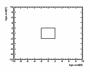
It is also possible to create/use 2d polygon cuts, either by specifying the parameters and (closed) polygon points:

  CUT:
    Cut2D(gHead.bgo.q[0], gHead.bgo.q[1], -2,-2, -2,2, 2,2, 2,-2, -2,-2)

This would create the following cut:

Alternatively, one may pre-define and then re-use graphical cuts using the “CMD:” option (see next).

1. CMD: Evaluates a series of commands in CINT.

The succeeding lines are a series of C++ statements to be evaluated literally in the CINT interpreter, closed by a line containing only “END”. Any objects created within these statements will become available for use in future commands throughout the definition file. Note that each file should only contain one “CMD:” statement (if it contains any), and that it should be the first “active” code within the file. As an example, we could use “CMD:” to define a graphical cut:

  CMD:
    TCutG cutg("cutTest",7);
    cutg.SetVarX("");
    cutg.SetVarY("");
    cutg.SetTitle("Graph");
    cutg.SetFillColor(1);
    cutg.SetPoint(0,37.8544,70.113);
    cutg.SetPoint(1,25.5939,41.5819);
    cutg.SetPoint(2,54.9042,28.0226);
    cutg.SetPoint(3,83.0651,35.3672);
    cutg.SetPoint(4,81.5326,53.1638);
    cutg.SetPoint(5,59.3103,79.1525);
    cutg.SetPoint(6,37.8544,70.113);
  END

This cut is then available in future statements; for example to create a Cut2D object to be applied to a histogram

  SUMMARY:
    ("bgo_ecal", "Bgo energies [singles]", 256, 0, 4096)
    rootana::gHead.bgo.ecal 
    30
  CUT:
    Cut2D(gHead.bgo.ecal[0], gHead.bgo.ecal[1], cutg)

The above example would apply the graphical cut “cutg” defined in the “CMD:” statement to the “bgo_ecal” histogram.

With combinations of the above commands, you should hopefully be able to define any histogram-related objects you will need in the online analyzer without ever having to touch the source code. A few more notes about histogram definition files:

• There are five global instances of “top-level” classes which encapsulate all of the relevant data in the experiment. Each class corresponds to a different event type, and is mapped to a different ROOT tree in the output file. As you may have noticed in the examples, these will need to prefix any parameters to be displayed in histograms. They are:
  1. rootana::gHead - “Head” (gamma) singles event
  2. rootana::gTail - “Tail” (heavy-ion( singles event
  3. rootana::gCoinc - Coincidence event
  4. rootana::gHeadScaler - “Head” (gamma) scaler event
  5. rootana::gTailScaler - “Tail” (heavy-ion) scaler event

• White-space is ignored, though good indention improves readability immensely.

• The # character denotes a comment, all characters on the same line coming after a # are ignored:

  # IGNORE THIS HEADER STATEMENT #
  TH1D: #Ignore this descriptive comment also...
  

• The run-time parsing is done using CINT via the gROOT->ProcessLine() and gROOT->ProcessLineFast() commands. These have very little native error handling. Some support has been added in the DRAGON analyzer to “gracefully” handle common errors when detectable; for example, skipping the current definition and moving onto others, but alerting the user. If you find a case where you feel the error handling could be improved (in particular, where a mistake in the script file causes a crash or un-reported failure), do not hesitate to alert the developers.

Once started, the online analyzer simply runs in the background to receive, match, and analyze events coming from the two separate front-ends. The analyzed data are then summarized in the histograms requested by the user as outlined in the proceeding paragraphs. As mentioned, roody can be used to visualize the histograms as data is coming in. To start roody, you will need to specify the host and port of the histogram server. Usually this means, the following:

roody -Plocalhost:9091

if running locally from the back-end host, or

roody -Pdaenerys.triumf.ca:9091

if running remotely. Roody is a graphical program, and as such its use is fairly intuitive. When you start the program, you should see a graphical outline of the histograms and directory structure you created in your hist definitions file that looks something like this:

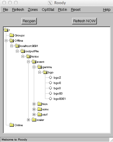
Simply double click on a histogram icon, and a ROOT canvas will be created showing the histogram. You can play around with the menu bars to explore other options, such as canvas refresh rate and canvas configuration.